Integrated likelihood methods for eliminating nuisance parameters
The process of inferring conclusions from experimental observations often requires the construction and evaluation of a likelihood function, which gives the probability, or probability density, of the observed data given a particular statistical model.
The likelihood function forms the basis for many statistical inference techniques. For example, one could estimate the parameters of a model by maximizing the likelihood. The problem is that likelihood functions frequently contain more parameters than we care about. The inexplicable or uninteresting noise that buffets processes of interest has to be parameterized and accounted for in the likelihood function. As Berger, Liseo, and Wolpert discuss in this paper, the existence of so-called ‘nuisance parameters’ severely hampers inference in many cases. The authors review a few of the common frequentist techniques for dealing with nuisance parameters in likelihood functions, but fall strongly in favor of integrating the likelihood function over the nuisance parameters. Although this method has a Bayesian flavor to it, the authors emphasize the practical benefits of integrated likelihoods, even for statisticians with more frequentist leanings.
[This post previously appeared in klogw.org].
Berger et al. present a number of scenarios where an integrated likelihood function forms a more robust basis for inference than the frequentist candidates. The benefits of using an integrated likelihood are well demonstrated in Example 4 of the paper, which involves estimating a parameter from samples drawn from a binomial distribution. This example is explored in this Jupyter notebook.
Estimation with binomial samples
Imagine that we’ve been challenged by a friend to estimate the number of times a coin has been flipped in a series of independent sessions, but(!) we’re only told how many times the coin landed on heads. In each session, the coin is flipped N times, heads appears with a probability p, and both are unknown. How can we estimate N? The binomial distribution is the natural probabilistic model for this situation, and we can use it to construct a likelihood function for N given the number of times heads is drawn with p as the nuisance parameter. The example in the paper considers five sessions, with the number of heads being 16, 18, 22, 25, and 27 for each session. This example, including equations and code, is worked through in detail here. For this case, the fulltwo-dimensional likelihood surface looks like this:
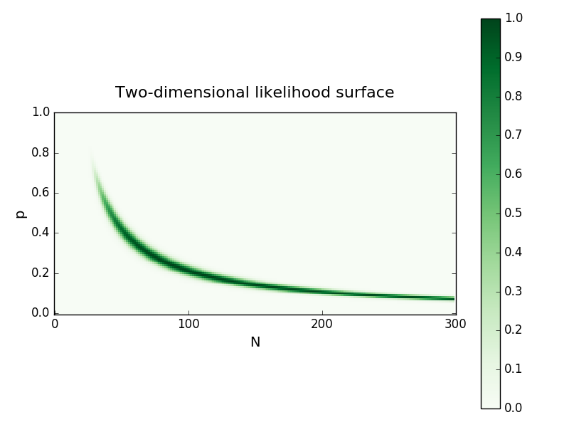
One way to estimate N is to maximize the two-dimensional likelihood, then record the value of N and discard the value of p. This is equivalent to maximizing the ‘profile likelihood’ of N: the one-dimensional projection of the likelihood surface over the values of p that maximize the likelihood for a given value of N. An alternative way to reduce the dimensionality of the full likelihood is to condition it on the sufficient statistic of the data, creating a ‘conditional likelihood’. Instead, Berger et al. recommend integrating the likelihood surface over p, which we can approximately think of as giving us the probability of observing N irrespective of the value of p. These dimensionality-reduced likelihoods are shown below:
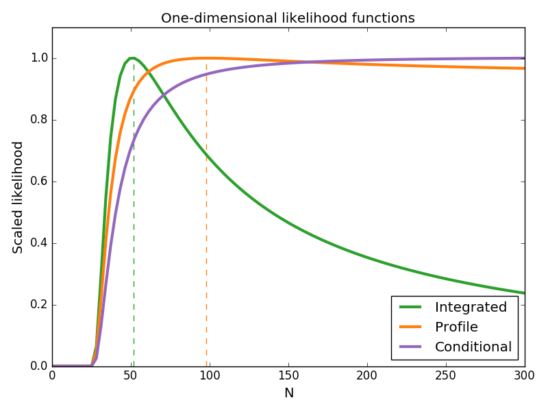
These three methods for eliminating the nuisance parameter p produce strikingly different likelihoods. As the conditional likelihood increases monotonically with N—without limit—it provides no basis for maximum likelihood estimation. While both the integrated and profile likelihoods have well defined maxima, the integrated likelihood has a maximum roughly half that of profile likelihood (shown in dotted lines). But which estimate is ‘better’? The curvature of the (log) likelihoods around the maximum is related to the uncertainty in our estimate of N. The fact that the integrated likelihood is more tightly peaked than the profile likelihood indicates that the maximum likelihood estimate is more robust than the estimate from the profile likelihood. As shown in Table 1 of the paper, repeating the entire coin flipping challenge and estimating N from the maximum of the profile likelihood produces a spread of estimates that is almost ten times as wide as the different estimates from the integrated likelihood. Therefore, in this case, the integrated likelihood is more practical than the conditional and profile likelihoods.